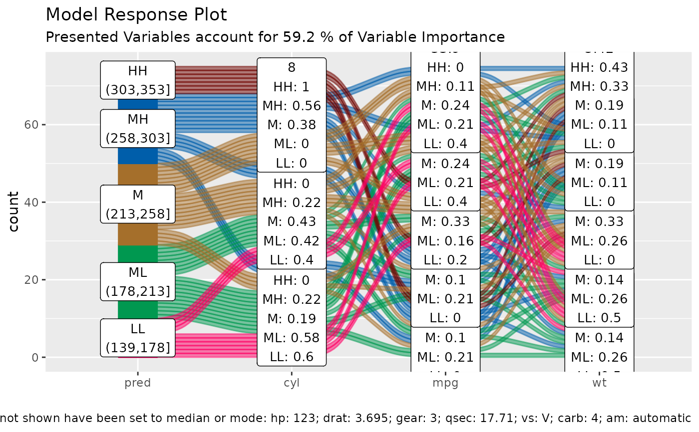
alluvial plots are capable of displaying higher dimensional data
on a plane, thus lend themselves to plot the response of a statistical model
to changes in the input data across multiple dimensions. The practical limit
here is 4 dimensions. We need the data space (a sensible range of data
calculated based on the importance of the explanatory variables of the model
as created by get_data_space and the predictions
returned by the model in response to the data space.
Usage
alluvial_model_response(
  pred,
  dspace,
  imp,
  degree = 4,
  bin_labels = c("LL", "ML", "M", "MH", "HH"),
  col_vector_flow = c("#FF0065", "#009850", "#A56F2B", "#005EAA", "#710500", "#7B5380",
    "#9DD1D1"),
  method = "median",
  force = FALSE,
  params_bin_numeric_pred = list(bins = 5),
  pred_train = NULL,
  stratum_label_size = 3.5,
  ...
)
Arguments
- pred
vector, predictions, if method = 'pdp' use
get_pdp_predictionsto calculate predictions- dspace
data frame, returned by
get_data_space- imp
dataframe, with not more then two columns one of them numeric containing importance measures and one character or factor column containing corresponding variable names as found in training data.
- degree
integer, number of top important variables to select. For plotting more than 4 will result in two many flows and the alluvial plot will not be very readable, Default: 4
- bin_labels
labels for prediction bins from low to high, Default: c("LL", "ML", "M", "MH", "HH")
- col_vector_flow,
character vector, defines flow colours, Default: c('#FF0065','#009850', '#A56F2B', '#005EAA', '#710500')
- method,
character vector, one of c('median', 'pdp')
- median
sets variables that are not displayed to median mode, use with regular predictions
- pdp
partial dependency plot method, for each observation in the training data the displayed variable as are set to the indicated values. The predict function is called for each modified observation and the result is averaged, calculate predictions using
get_pdp_predictions
. Default: 'median'
- force
logical, force plotting of over 1500 flows, Default: FALSE
- params_bin_numeric_pred
list, additional parameters passed to
manip_bin_numericswhich is applied to the pred parameter. Default: list( bins = 5, center = T, transform = T, scale = T)- pred_train
numeric vector, base the automated binning of the pred vector on the distribution of the training predictions. This is useful if marginal histograms are added to the plot later. Default = NULL
- stratum_label_size
numeric, Default: 3.5
- ...
additional parameters passed to
alluvial_wide
Details
this model visualisation approach follows the "visualising the model in the dataspace" principle as described in Wickham H, Cook D, Hofmann H (2015) Visualizing statistical models: Removing the blindfold. Statistical Analysis and Data Mining 8(4) <doi:10.1002/sam.11271>
Examples
df = mtcars2[, ! names(mtcars2) %in% 'ids' ]
m = randomForest::randomForest( disp ~ ., df)
imp = m$importance
dspace = get_data_space(df, imp, degree = 3)
pred = predict(m, newdata = dspace)
alluvial_model_response(pred, dspace, imp, degree = 3)


# partial dependency plotting method
if (FALSE) { # \dontrun{
 pred = get_pdp_predictions(df, imp
                            , .f_predict = randomForest:::predict.randomForest
                            , m
                            , degree = 3
                            , bins = 5)


 alluvial_model_response(pred, dspace, imp, degree = 3, method = 'pdp')
 } # }
# partial dependency plotting method
if (FALSE) { # \dontrun{
pred = get_pdp_predictions(df, imp
, .f_predict = randomForest:::predict.randomForest
, m
, degree = 3
, bins = 5)
alluvial_model_response(pred, dspace, imp, degree = 3, method = 'pdp')
} # }